BioQC-kidney: The kidney expression example
2021-08-24
BioQC.RmdIntroduction
In this vignette, we demonstrate the use of BioQC with a case study where mouse kidney samples were profiled for gene expression. Results of BioQC pointed to potential tissue heterogeneity caused by pancreas contamination which was confirmed by qRT-PCR experiments.
Importing the data
Let’s first load the BioQC signatures using readGmt:
library(BioQC)
gmtFile <- system.file("extdata/exp.tissuemark.affy.roche.symbols.gmt",
                        package="BioQC")
gmt <- readGmt(gmtFile)
The example data for this vignette is shipped as part of the BioQC package. Alternatively, it is available in the GitHub repository. The expression data is stored in a ExpressionSet.
file <- system.file("extdata/kidney_example.rda", package="BioQC")
load(file)
print(eset)
The dataset contains expression of 34719 genes in 25 samples. The expression profile was normalized with RMA normalization. The signals were also log2-transformed; however, this step does not affect the result of BioQC since it is essentially a non-parametric statistical test.
Running BioQC
Next we run the core function of the BioQC package, wmwTest, to perform the analysis.
system.time(bioqcRes <- wmwTest(eset, gmt,
                                 valType="p.greater"))
## user system elapsed
## 0.864 0.016 0.880The function returns one-sided \(p\)-values of Wilcoxon-Mann-Whitney test.
For better visualization we * filter the p-value matrix (a sensible cutoff depends on the actual dataset and the expected signatures); * transform the p-values using \(|\log_{10} p|\). We refer to thse transformed values as BioQC score.
bioqcResFil <- filterPmat(bioqcRes, 1E-6)
bioqcAbsLogRes <- absLog10p(bioqcResFil)
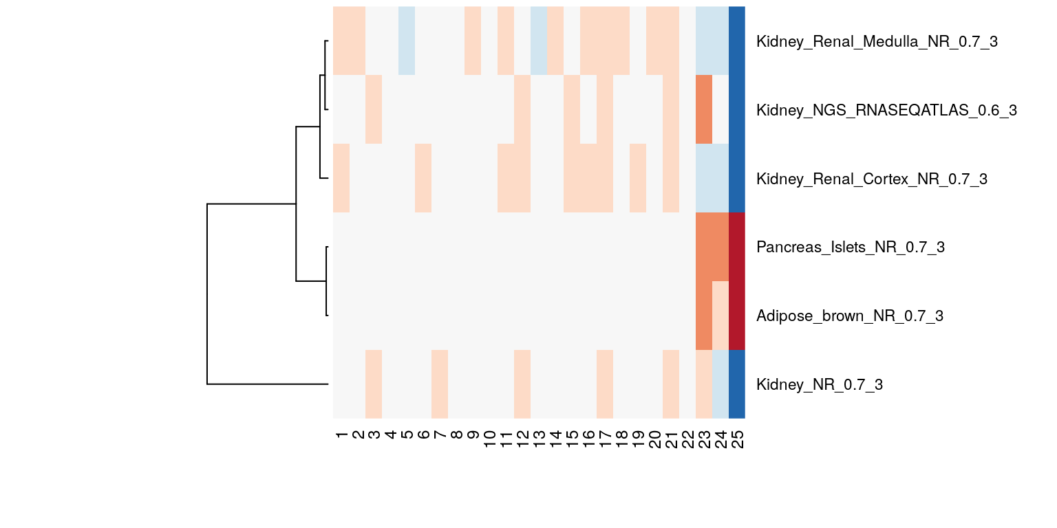
We inspect the BioQC scores by visualizing them as Heatmap. By closer examination we find that the expression of pancreas and adipose specific genes is significantly enriched in samples 23-25:
library(RColorBrewer)
heatmap(bioqcAbsLogRes, Colv=NA, Rowv=TRUE,
        cexRow=0.85, scale="row",
        col=rev(brewer.pal(7, "RdBu")),
        labCol=1:ncol(bioqcAbsLogRes))
BioQC scores (defined as abs(log10(p))) of the samples visualized in heatmap. Red and blue indicate high and low scores respectively.
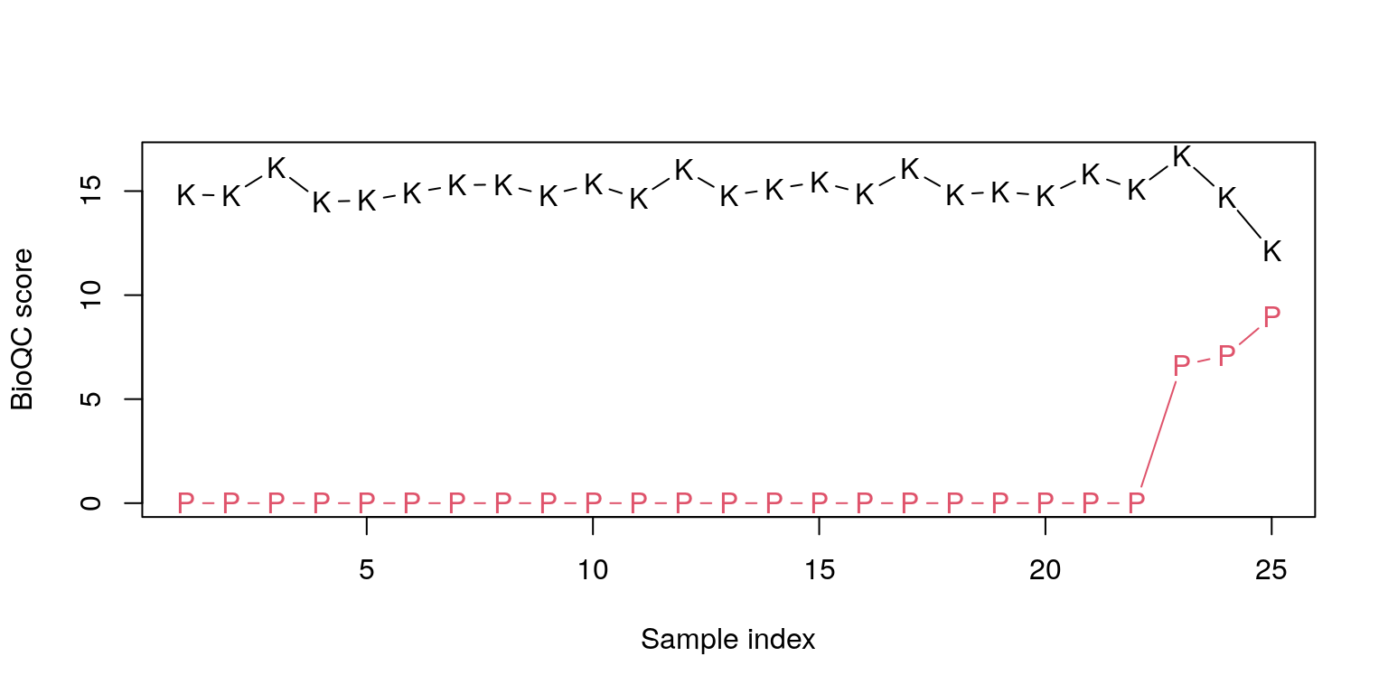
Visual inspection reveals that there might be contaminations in samples 23-25, potentially by pancreas and adipose tissue.
filRes <- bioqcAbsLogRes[c("Kidney_NGS_RNASEQATLAS_0.6_3",
                           "Pancreas_Islets_NR_0.7_3"),]
matplot(t(filRes), pch=c("K", "P"), type="b", lty=1L,
        ylab="BioQC score", xlab="Sample index")
BioQC scores (defined as abs(log10(p))) of the samples. K and P represent kidney and pancreas signature scores respectively.
Validation with quantitative RT-PCR
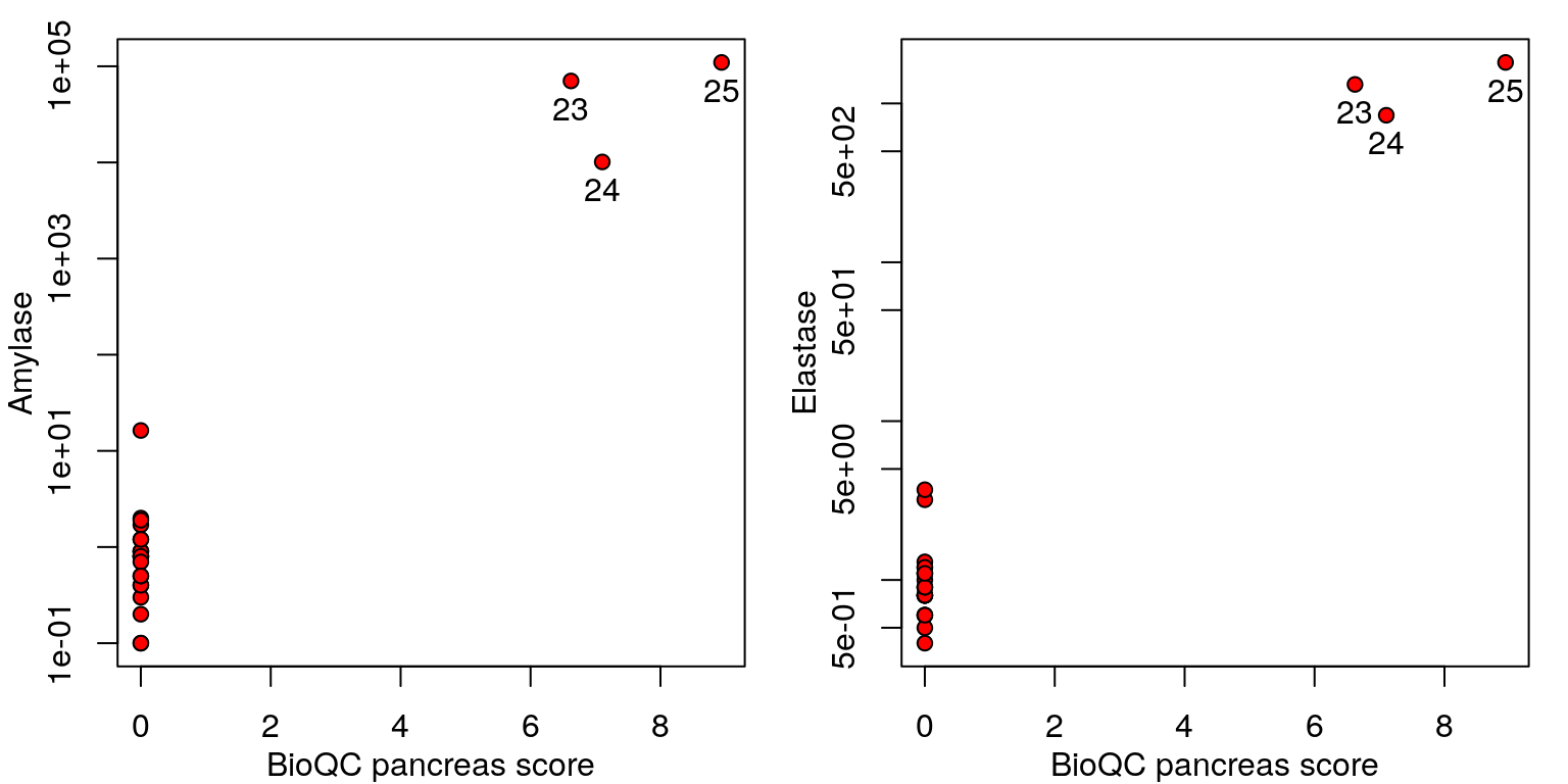
To confirm the hypothesis generated by BioQC, we performed qRT-PCR experiments to test two pancreas-specific genes’ expression in the same set of samples. Note that the two genes (amylase and elastase) are not included in the signature set provided by BioQC.
The results are shown in the figure below. It seems likely that sample 23-25 are contaminated by nearby pancreas tissues when the kidney was dissected. Potential contamination by adipose tissues remains to be tested.
amylase <- eset$Amylase
elastase <- eset$Elastase
pancreasScore <- bioqcAbsLogRes["Pancreas_Islets_NR_0.7_3",]
par(mfrow=c(1,2), mar=c(3,3,1,1), mgp=c(2,1,0))
plot(amylase~pancreasScore, log="y", pch=21, bg="red",
     xlab="BioQC pancreas score", ylab="Amylase")
text(pancreasScore[23:25],amylase[23:25], 23:25, pos=1)
plot(elastase~pancreasScore, log="y", pch=21, bg="red",
     xlab="BioQC pancreas score", ylab="Elastase")
text(pancreasScore[23:25],elastase[23:25], 23:25, pos=1)
Correlation between qRT-PCR results and BioQC pancreas score
Impact of sample removal on differential gene expression analysis
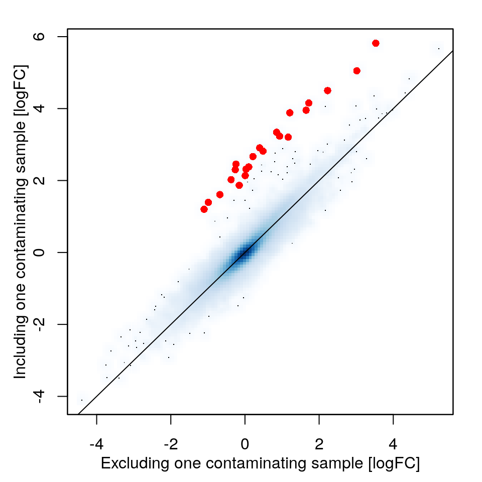
In this study, four mice of the FVB/NJ strain received nephrectomy operation and treatment of Losartan, an angiotensin II receptor antagonist drug, and four mice reveiced an sham operation and Losartan. Within the Nephrectomy+Losartan group, one sample (index 24) is possibly contaminated by pancreas. Suppose now we are interested in the differential gene expression between the conditions. We now run the analysis twice, once with and once without the contaminated sample, to study the impact of removing heterogenous samples detected by BioQC.
isNeph <- with(pData(eset), Strain=="FVB/NJ" &
                 TREATMENTNAME %in% c("Nephrectomy-Losartan", "Sham-Losartan"))
isContam <- with(pData(eset), INDIVIDUALNAME %in% c("BN7", "FNL8", "FN6"))
esetNephContam <- eset[,isNeph]
esetNephExclContam <- eset[, isNeph & !isContam]
getDEG <- function(eset) {
  group <- factor(eset$TREATMENTNAME, levels=c("Sham-Losartan","Nephrectomy-Losartan"))
  design <- model.matrix(~group)
  colnames(design) <- c("ShamLo", "NephLo")
  contrast <- makeContrasts(contrasts="NephLo", levels=design)
  exprs(eset) <- normalizeBetweenArrays(log2(exprs(eset)))
  fit <- lmFit(eset, design=design)
  fit <- contrasts.fit(fit, contrast)
  fit <- eBayes(fit)
  tt <- topTable(fit, n=nrow(eset))
  return(tt)
}

esetNephContam.topTable <- getDEG(esetNephContam)
esetNephExclContam.topTable <- getDEG(esetNephExclContam)
esetFeats <- featureNames(eset)
esetNephTbl <- data.frame(feature=esetFeats,
                          OrigGeneSymbol=esetNephContam.topTable[esetFeats,]$OrigGeneSymbol,
                          GeneSymbol=esetNephContam.topTable[esetFeats,]$GeneSymbol,
                          Contam.logFC=esetNephContam.topTable[esetFeats,]$logFC,
                          ExclContam.logFC=esetNephExclContam.topTable[esetFeats,]$logFC)
par(mfrow=c(1,1), mar=c(3,3,1,1)+0.5, mgp=c(2,1,0))
with(esetNephTbl, smoothScatter(Contam.logFC~ExclContam.logFC,
                                xlab="Excluding one contaminating sample [logFC]",
                                ylab="Including one contaminating sample [logFC]"))
abline(0,1)
isDiff <- with(esetNephTbl, abs(Contam.logFC-ExclContam.logFC)>=2)
with(esetNephTbl, points(Contam.logFC[isDiff]~ExclContam.logFC[isDiff], pch=16, col="red"))
Log2 fold change (logFC) values reported by limma with one contaminated sample included (y-axis) or excluded (x-axis). Genes strongly affected by the contamination are indicated by red dots.
diffTable <- esetNephTbl[isDiff,]
diffGenes <- unique(diffTable[,"GeneSymbol"])
pancreasSignature <- gmt[["Pancreas_Islets_NR_0.7_3"]]$genes
diffGenesPancreas <- diffGenes %in% pancreasSignature
diffTable$isPancreasSignature <- diffTable$GeneSymbol %in% pancreasSignature
colnames(diffTable) <- c("Probeset", "GeneSymbol", "Human ortholog",
                         "Log2FC", "Log2FC (excl. contam.)",
                         "IsPancreasSignature")
diffTable <- diffTable[order(diffTable$Log2FC, decreasing=TRUE),]
We found that 22 probesets representing 17 genes are associated with much stronger expression changes if the contaminated sample is not excluded (table below). Not surprisingly almost all of these genes are highly expressed in normal human pancreas tissues, and 13 genes belong to the pancreas signature used by BioQC.
In summary, we observe that tissue heterogeneity can impact down-stream analysis results and negatively affect reproducibility of gene expression data if it remains overlooked. It underlines again the value of applying BioQC as a first-line quality control tool.
R Session Info
## R version 4.1.0 (2021-05-18)
## Platform: x86_64-pc-linux-gnu (64-bit)
## Running under: Ubuntu 20.04.2 LTS
##
## Matrix products: default
## BLAS/LAPACK: /usr/lib/x86_64-linux-gnu/openblas-pthread/libopenblasp-r0.3.8.so
##
## locale:
##  [1] LC_CTYPE=en_US.UTF-8       LC_NUMERIC=C
##  [3] LC_TIME=en_US.UTF-8        LC_COLLATE=en_US.UTF-8
##  [5] LC_MONETARY=en_US.UTF-8    LC_MESSAGES=C
##  [7] LC_PAPER=en_US.UTF-8       LC_NAME=C
##  [9] LC_ADDRESS=C               LC_TELEPHONE=C
## [11] LC_MEASUREMENT=en_US.UTF-8 LC_IDENTIFICATION=C
##
## attached base packages:
## [1] stats     graphics  grDevices utils     datasets  methods   base
##
## other attached packages:
## [1] limma_3.49.4        RColorBrewer_1.1-2  BioQC_1.21.4
## [4] Biobase_2.53.0      BiocGenerics_0.39.2 knitr_1.33
##
## loaded via a namespace (and not attached):
##  [1] Rcpp_1.0.7         edgeR_3.35.0       magrittr_2.0.1     lattice_0.20-44
##  [5] R6_2.5.0           ragg_1.1.3         rlang_0.4.11       fastmap_1.1.0
##  [9] highr_0.9          stringr_1.4.0      tools_4.1.0        grid_4.1.0
## [13] xfun_0.25          KernSmooth_2.23-20 jquerylib_0.1.4    htmltools_0.5.1.1
## [17] systemfonts_1.0.2  yaml_2.2.1         digest_0.6.27      rprojroot_2.0.2
## [21] pkgdown_1.6.1.9001 crayon_1.4.1       textshaping_0.3.5  sass_0.4.0
## [25] fs_1.5.0           memoise_2.0.0      cachem_1.0.5       evaluate_0.14
## [29] rmarkdown_2.10     stringi_1.7.3      compiler_4.1.0     bslib_0.2.5.1
## [33] desc_1.3.0         locfit_1.5-9.4     jsonlite_1.7.2